Newtons laws of motion may be applicable ideally for bodies belonging to identified systems, however in fluid dynamics, for a control fluid volume in motion, Reynolds transport theorem becomes more appropriate. Learn more.
Reynolds Transport Theorem
When we say dynamics, to us, it relates to the study of the states of motion under the influence of external forces and moments. We have learned Newton’s laws of motion quite well: a fluid system should adhere to the three laws of motion as per Newtonian mechanics.
According to Newton’s third law of motion, every action is accompanied by an equal and opposite reaction. The action and reaction taking place between two or more bodies is particularly governed by this law. While studying fluid flow dynamics, the law can be also applied for fluid elements, where their mutual interactions involve actions and reactions which are oppositely directed. For example the thrust exerted by a boat jet engine over a volume of water (fluid) through a confined channel, generates equal and opposite thrust from this volume of fluid over the jet engine.
However the above law may be true only for bodies or systems with identified or fixed measurable parameters. Considering a control volume of fluid (since unidentified masses of fluid may undergo constant deformation and transformation while in motion), the above laws of physics can be extended through Reynolds transport theorem.
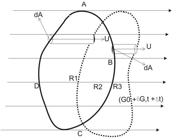
Referring to the figure above, we see the following:
-
A control volume of fluid in motion ABCD at some point of time t.
-
Due to motion, the control volume takes a new position (shown by dotted lines) after a time t + δt.
-
The position of volume in the flow field is expressed by G and also the extensive property N, which depends upon the mass of the fluid, becomes the function of intensive property denoted as n, independent of the mass of the fluid.
Now as per the definition of Reynolds transport theorem, for a system the rate of change of the extensive property N must equal the total effluence across the control surface and within the control volume.
Let’s evaluate and prove the above theorem.
Again referring to the diagram alongside we can write:
N = ∫ n__ρ dV = N (G, t),
Whence, (dN/dt)s = DN/Dt = lim (∆t→0) {N(G0 + δG,t + δt) – N(G0,t)} / δt
In the above equation G0 and G0 + δG identify the locations of the volumes at t and t + δt respectively.
Adding and deducting the expression _N(_G0,t + δt) in the term below the limit and repositioning them as two expressions we get:
lim (∆t→0) {N(G0,t + δt) – N(G0,t)} – N(G0,t)} / δt = ∂/∂t ∫ nρ dV
The above equation suggests that the local rate of change of N and N(G0 + δG,t + δt) – N(G0,t) / δt inside the control volume is = N3 + N1, where N1 and N3 indicate the magnitudes of N for the areas R1 and R2 respectively, the area R2 being common to both the locations.
So, N3 = ∫ nρ (dA.Uδt) = ∫CDA nρ dt (U.dA)
And, – N1 = ∫ABC nρδt (U.dA);
therefore, N3 – N1 = ∫ABCD nρδt (U.dA)
When the second limit-term is reduced to ∫ n(ρU.dA);
Finally we evaluate Reynolds transport theorem through the following expression:
DN/Dt = ∫CS n(ρU.dA) + ∂/∂t ∫CV nρ dV where CS is the surface bounding the system and CV is the volume of the system.
In the above expression when N is the mass as per the law of conservation, the LHS disappears and the equation becomes:
∫CS ρU.dA + ∂/∂t ∫CV ρ dV = 0
The above equation of continuity further shortens to a more recognizable form as:
_◊.(_ρU) + ∂ρ/∂t = 0 >
References
Book: Engineering Fluid Mechanics By K.L. Kumar,
The Reynolds Transport Theorem - eng.fsu.edu
Derivation of Reynolds Transport Theorem - web.ce.metu.edu