Introduction to Pro-mechanica, FEA, FEM. Pro-mechanica Tutorial
The two terms FEAand FEM are often used interchangeably. But there are some differences in the terms.
FEM or Finite Element Method is a mathematical method for solving physical problems. FEM evaluates solutions at various points called nodes. There are three methods of FEM, namely non-variational method (Ritz), the residual method (Galerkin) & the variational method (Rayleigh-Ritz).
FEA or Finite Element Analysis on the other hand is the implementations of FEM. There are numerous different software programs available to implement FEM, known as FEA software.
Basics of FEA
The whole process of any FEA could be divided into three broad sections irrespective of which software you use:
1. Preprocessing: When you do an analysis you have to do modeling and meshing. In pro-mechanica, analysis model is created in pro-engineer standard module and then the model of part or assembly is brought to pro-mechanica module. In pro-mechanica module the model is meshed and the boundary conditions are applied.
New terms:
Meshing: The process of breaking the geometric model into small pieces in order to create nodes and elements is called meshing. In other words meshing is the process of converting the geometric model to a FEA model.
Boundary Conditions: In order to solve a FEA problem you have to apply force (these force could be structural, thermal, magnetic or of any form) and you have to resist at some points of the model from the effects generated by these forces. For example to see the stress in a cube you may think of applying force at the top surface and can constrain it at the parallel bottom surface. These set of loads and constraints are called boundary conditions.
2. Solving: After pre-processing we have to use a solver to find solution out of the FEA problem. In pro-mechanica we could either use the native pro-mechanica solver or can export or save the pre-processed mesh for solving with other external solver like ANSYS, NASTRAN etc.
3. Post-Processing: After solving you view the results of your FEA problem. This section is called post-processing. Here we can see different types of plots and graphs of the result.
Getting Started with Pro-Mechanica
In order to run an analysis you have to model the required geometry using standard pro-engineer module. Save it and follow the path: Applications>Mechanica
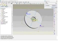
You may see a screen like this:
There will be a small dialogue box at the top right corner of the screen named “Model Type”, in this dialogue box we can select the mode of the analysis (like, structural or thermal).
By checking the box near FEM mode you can tell pro-mechanica whether you want to create only the mesh in mechanica or you want to solve also in pro-mechanica.
By clicking the “Advanced “button you can select the sub type of the analysis (For example, you can select either 3D or 2D plane stress or 2D plain strain or 2D Axisymmetric.
In pro-mechanica we can solve either structural or thermal problems. In both the cases the following subtypes of model are possible:
- 3D: The whole 3D geometry is converted to FEA mesh. The approach is quite simple but it requires more computer resources.
- 2D Plane stress: In a 3D problem if the loads and displacements are in XY plane and the part is a thin, flat plate kind of model (t<
To solve using this method you have to select the surface which is in XY plane and also the co-ordinate system with respect to which the plane is in XY.
- 2D plane strain: When in a 3D model the strain developed perpendicular to a certain surface is zero then we can solve the problem by plane strain method. In plane strain problem the structure should substantially long (h»a, b) and Geometry, loads and displacements should be in XY plane. In case of an assembly all the components should in same Z depth.
Long tube carrying water is an example of plane strain problem.
To solve using this method you have to select the surface which is in XY plane and also the co-ordinate system.
- 2D Axisymmetric: If by revolving a slice of 2D model to 360 degree around y axis the 3D model is formed and the geometry, loads and displacements of the slice is at positive side XY plane then the problem could be solved by this approach.
Suppose we have a circular plate with a hole at the centre and the plate is under uniform loading at the top surface, and then we can use the 2D section (for analysis) by revolving which we could obtain the plate
The 3d, plane stress, plane strain and axisymmetric problems will be discussed in depth with example in other parts of the tutorial.
Read More About FEM and FEA
Here some additional resources explaining FEM and FEA:
What is the FEM? https://web.mit.edu/16.810/www/16.810_L4_CAE.pdf
Introduction to Finite Element Analysis: https://www.sv.vt.edu/classes/MSE2094_NoteBook/97ClassProj/num/widas/history.html
Introduction to FEA or FEM: https://www.cs.ubbcluj.ro/~alibal/Teaching/Simulation/FEA_FEM.pdf
This post is part of the series: Pro-Mechanica Tutorial
Pro-mechanica is a FEA module of pro-engineer. If you complete reading this series and do practice as required then you will be able to do analysis using pro-mechanica, of course you should have basic knowledge of pro-engineer or other 3D cad package.
- Pro-Mechanica Tutorial Part 1: Introduction to FEA
- Pro-Mechanica Tutorial Part 2: AutoGEM & Meshing
- Pro-Mechanica Tutorial Part 3: Structural Loads
- Pro-Mechanica Tutorial Part 4: Thermal Loads
- Pro-Mechanica Tutorial Part 5: Thermal Constraints
- Pro-Mechanica Tutorial Part 6: Structural Constraints
- Pro Engineer Mechanica Tutorial Part 7: Analysis and Design Studies
- Pro-Mechanica Tutorial Part 8: Reviewing FEA Results